
Currency baskets, stablecoins, libra etc (Part 1)
Published:
This note is based on our paper Giudici et al. (2021).
Stablecoins have become a major talking point in the cryptoasset domain. From the private sector, Facebook, amongst numerous others, have announced plans for their own privately issued stablecoin. In the most recent iteration of Facebooks proposition, the idea is to supply digital tokens that are pegged to major currencies, i.e. LibraUSD would be pegged to the US dollar. In addition, there will be another token whose value is derived from a weighted basket of the currencies provided on the platform. The exact composition of this basket and its targeted exchange rate is unspecified. With this research we ask the optimal structure of this basket. For this, we start from the assumption that the objective is to devise a digital currency whose exchange rate fluctuations are minimised against several currencies of the worlds major currencies.
To devise a minimum varying currency basket we use a methodology proposed by Hovanov et al. (2004). First, we obtain our FX rates. As a benchmark we start from the 5 currencies used in the IMFs SDR currency basket.
| USD | CNY | EUR | GBP | JPY | |
|---|---|---|---|---|---|
| USD | 1.0000 | 0.1208226 | 0.8707009 | 1.423488 | 0.0075563 |
| CNY | 8.2766 | 1.0000000 | 7.2064432 | 11.781637 | 0.0625404 |
| EUR | 1.1485 | 0.1387647 | 1.0000000 | 1.634875 | 0.0086784 |
| GBP | 0.7025 | 0.0848778 | 0.6116674 | 1.000000 | 0.0053083 |
| JPY | 132.3400 | 15.9896576 | 115.2285590 | 188.384342 | 1.0000000 |
Hovanov et al. (2004) (herein HKS) show how to compute a invariant currency value index (ICVI) which is independent of base currency choice. Such that any set of foreign exchange rates can be converted to the index regardless of the base currency.
To convert exchange rates into a currency invariant index HKS utilize the fact that exchange rates are measured by a scale of ratios with a precision of a positive factor β, where β is defined as the geometric mean of the exchange rates.
where, cij denotes the exchange rates. We compute these values through time and for convenience work with the reduced (to the moment t=0) normalized value in exchange. Such that at date t=0 the value RNVali = 1. The reduced normalised values are shown in the table below:
| Date | USD | CNY | EUR | GBP | JPY | |
|---|---|---|---|---|---|---|
| 1286 | 2002-02-04 | 1.0000000 | 1.0000000 | 1.0000000 | 1.000000 | 1.000000 |
| 1300 | 2002-02-05 | 0.9957958 | 0.9957837 | 0.9991772 | 1.001607 | 1.007685 |
| 1314 | 2002-02-06 | 0.9957076 | 0.9957197 | 0.9990888 | 1.003362 | 1.006166 |
| 1329 | 2002-02-07 | 0.9967829 | 0.9967829 | 0.9964357 | 1.003168 | 1.006876 |
| 1343 | 2002-02-08 | 0.9960409 | 0.9960529 | 0.9928321 | 1.001854 | 1.013352 |
| 1381 | 2002-02-11 | 0.9995058 | 0.9995300 | 0.9931528 | 1.000502 | 1.007361 |
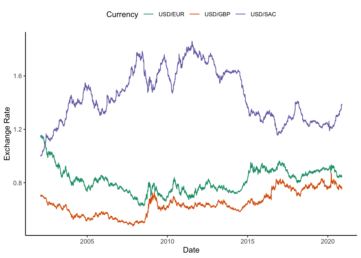
Over time these values look like:

The interpretation of the ICVI is that changes in value of the corresponding currencies can be assessed in the context of an average. Typically, we only measure performances of currencies against a numeraire (another currency or asset). By contrast, using the index, we would infer that the value of the dollar was rising on average against the currencies used in the computation of the geometric mean currency value. From our plot we observe the USD and GBP are the currencies that have appreciated the most against the average of our set of currencies, while the CNY, EUR and YEN have depreciated (on average) since 2002.
HKS go on to demonstrate how the index can be used to derive a minimum variance currency basket (MVCB) e.g. a stablecoin! The objective is to solve the optimal weights across the currencies.
Now we want to find the composition of the basket to generate ‘the most stable’ currency. The volatility of the currency invariant index time series is our target of stability i.e. the lower the volatility the more stable the currency. This can be framed as an optimisation problem:
where Ω is the covariance of the reduced normalised values. Computing this we find the weights to devise the minimum varying currency basket (stablecoin).
| USD | CNY | EUR | GBP | JPY | |
|---|---|---|---|---|---|
| Stablecoin | 0.168 | 0.194 | 0.235 | 0.191 | 0.212 |
| SDR | 0.420 | 0.110 | 0.310 | 0.080 | 0.080 |
The weights derived from the minimisation problem suggests that the distribution of the weights should be spread more evenly than those of the IMF SDRs. The heavier weighting on the dollar means fluctuations of SDRs will be positive correlated with those of the dollar, whereas the more diversified weight regime implied by the minimisation problem implies that the fluctuations of individual currencies in the basket offset one another. Working with the currency invariant indices is useful but what most people would be concerned with is the price of the stablecion (in dollars or any other currency).
To retrieve the price we need to obtain the quantities of each currency should be held, this is obtained through the following relation:
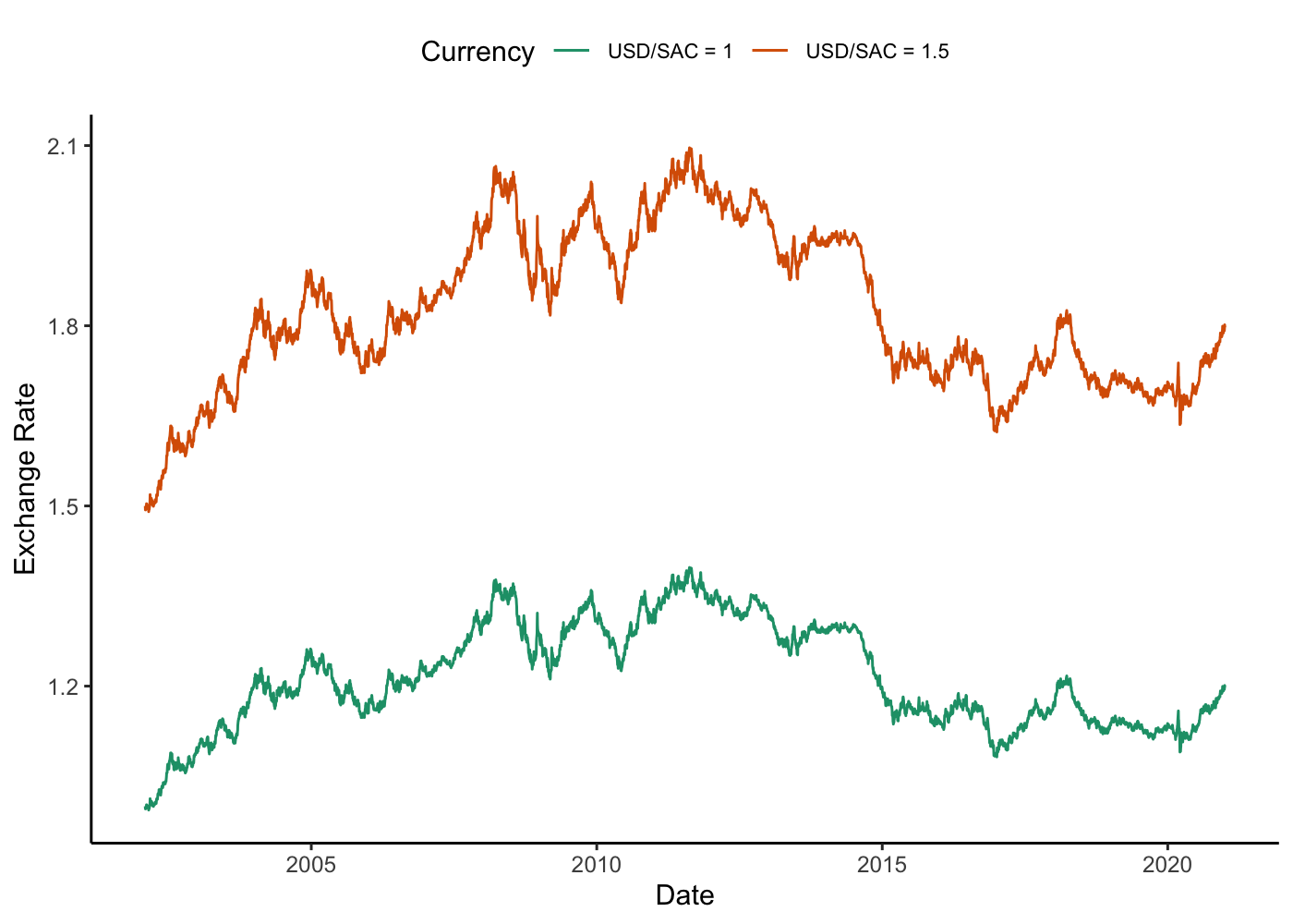
where μ is a scale factor that effectively determines the initial exchange rate between the stablecoin and a chosen currency, j. For example, if we we take μ = 1, 1 unit of stablecoin (SAC) will equal 1 unit of the second currenc e.g. USD. We start from 1SAC = 1USD. Note we can target any price and the same series will be replicated, but simply rescaled, such that we could choose any target price to start from. The plot below shows a rescaled version by 1.5.
How can this work in practice?
So far, HKS provide us a methodology to find a minimum varying currency basket, but the so far we only looked at the moethodology in a backward looking context. We don’t know how it would perform out-of-sample. As a simple exercise we compute weights based on a 30-day rolling window, then project the price over the next 30 days i.e. a we consider a scenario where an issuer of a weighted stablecion could update the weights every 30 days based on this methodology to keep the price as stable as possible. We then update μ in each window to be the last observed price of the previous window.
From the graph, the price of the stablecoin appears to follow a similar path to that of the historic price reconstruction done previously. If we look at the standard deviations of the series the rolling window series is more volatile (less stable), σr2 = 0.2, compared to the historical reconstruction, σh2 = 0.2. The series also runs countercyclical to the path followed by the Euro and Sterling, eluding to some notion that this asset could be used for hedging currency risks.
What else can we do?
The first step that one might think of is to add additional assets or currencies to the basket. In particular, since we are talking about stablecoins in the crypto domain we can see if we can construct a stable basket of cryptocurrencies. We strat with a basket of Bitcoin, EOS, Ethereum, Litecoin, Monero, Stellar and XRP.
Calculating the invariant indices we can plot them…
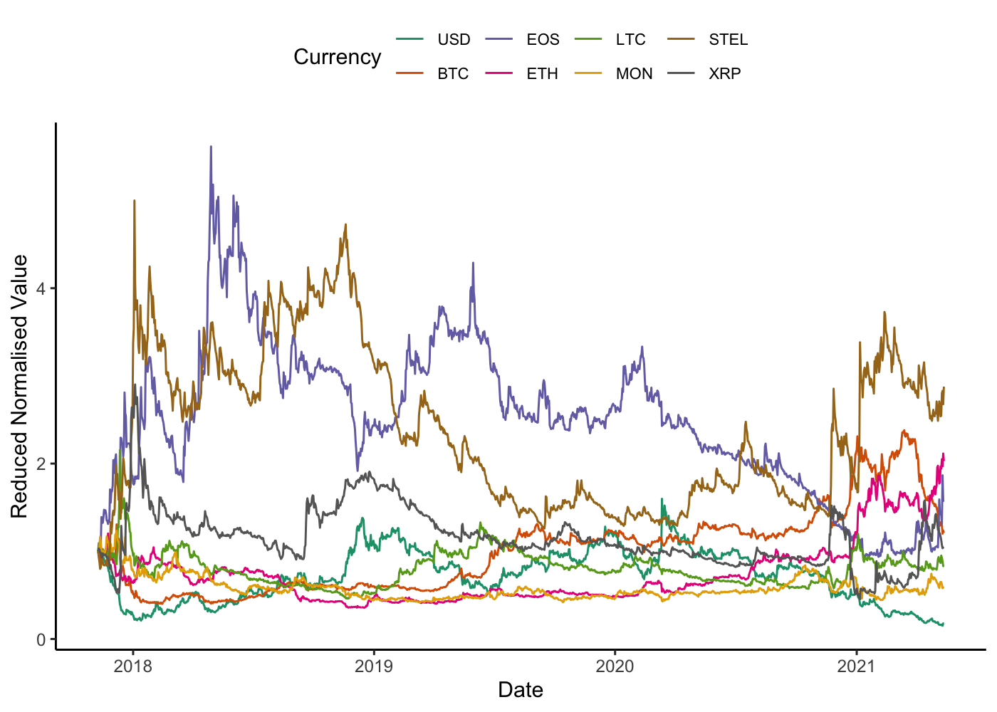
The picture is a different one to what we observed with major currencies, perhaps unsurprisingly as cryptocurrencies exhibit price dynamics markedly different from the standard currencies. However, could we construct something less volatile using these cryptocurrencies? Something of additional interest to note from the graph is that in 2021 the dollars has depreciated on average against all of the cryptocurrencies in the basket.
We construct our weighted average basket as before and this time inspect the correlations between the RNvals of the cryptocurrencies (+ dollar) in our basket and our weighted combination. The correlation between the stablecoin, denoted SAC, are relatively low with respect to other cryptocurrencies i.e. -> 0.
| USD | BTC | EOS | ETH | LTC | MON | STEL | XRP | SAC | |
|---|---|---|---|---|---|---|---|---|---|
| USD | 1.000 | -0.089 | 0.102 | -0.636 | -0.328 | -0.438 | -0.440 | 0.049 | 0.087 |
| BTC | -0.089 | 1.000 | -0.759 | 0.660 | 0.075 | -0.107 | -0.359 | -0.677 | 0.055 |
| EOS | 0.102 | -0.759 | 1.000 | -0.647 | -0.003 | -0.225 | 0.187 | 0.309 | 0.030 |
| ETH | -0.636 | 0.660 | -0.647 | 1.000 | 0.110 | 0.254 | 0.101 | -0.439 | 0.074 |
| LTC | -0.328 | 0.075 | -0.003 | 0.110 | 1.000 | 0.230 | -0.349 | -0.168 | 0.137 |
| MON | -0.438 | -0.107 | -0.225 | 0.254 | 0.230 | 1.000 | 0.000 | -0.053 | 0.192 |
| STEL | -0.440 | -0.359 | 0.187 | 0.101 | -0.349 | 0.000 | 1.000 | 0.429 | 0.029 |
| XRP | 0.049 | -0.677 | 0.309 | -0.439 | -0.168 | -0.053 | 0.429 | 1.000 | 0.077 |
| SAC | 0.087 | 0.055 | 0.030 | 0.074 | 0.137 | 0.192 | 0.029 | 0.077 | 1.000 |
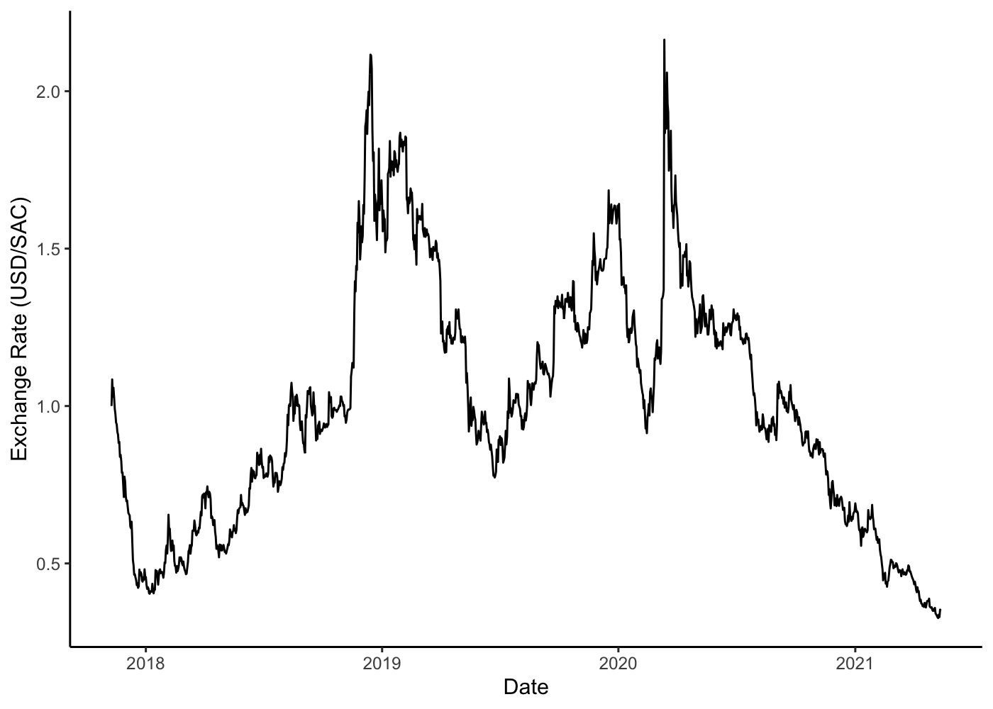
We can then plot the exchange rate of this crypto-based stablecoin against the dollar (again using μ = 1). The coefficient of variation of the crypto-based stablecoin is 0.4. Not as low that of a previously constructed stablecoin but nonetheless an improvement in volatility when compared to other cryptocurrencies. Bitcoin, for example, has a coefficient of variation of 1 during the same time period.
## [1] 0.3856767

## [1] 1.007508
There are several ways to go from here - one can think of ways to optimise which cryptocurrencies are best to have in the basket - or changing the criteria for currencies that should be in the basket that change over time or considering other assets to put in the basket. We will cover more in a second part to this.